Digit generator

Following tradition, as a tribute to pi day, I will attempt to recreate a particular visual representation of the digits of $\pi$. The original creation is due to Martin Krzywinski, and can be found here. The digits of $\pi$ were computed using the Chudnovsky algorithm. Due to the CPU-intensive nature of such a computation, I precomputed the digits and saved to them a file for reuse. This is less time consuming than computing the digits every time when visualizing them (or if you write buggy programs like I do). Below is the python script that computes the $n$ first digits of $\pi$ and saves as them to a file:

def pi_digits(n):
    """
    Computes PI using the Chudnovsky algorithm from
    http://stackoverflow.com/questions/28284996/python-pi-calculation
    """
 
    # Set precision
 
    getcontext().prec = n
 
    t = Decimal(0)
    pi = Decimal(0)
    d = Decimal(0)
 
    # Chudnovsky algorithm
 
    for k in range(n):
        t = ((-1)**k)*(factorial(6*k))*(13591409+545140134*k)
        d = factorial(3*k)*(factorial(k)**3)*(640320**(3*k))
 
        pi += Decimal(t) / Decimal(d)
 
    pi = pi * Decimal(12) / Decimal(640320**(Decimal(1.5)))
    pi = 1 / pi
 
    return str(pi)

Grid visualization

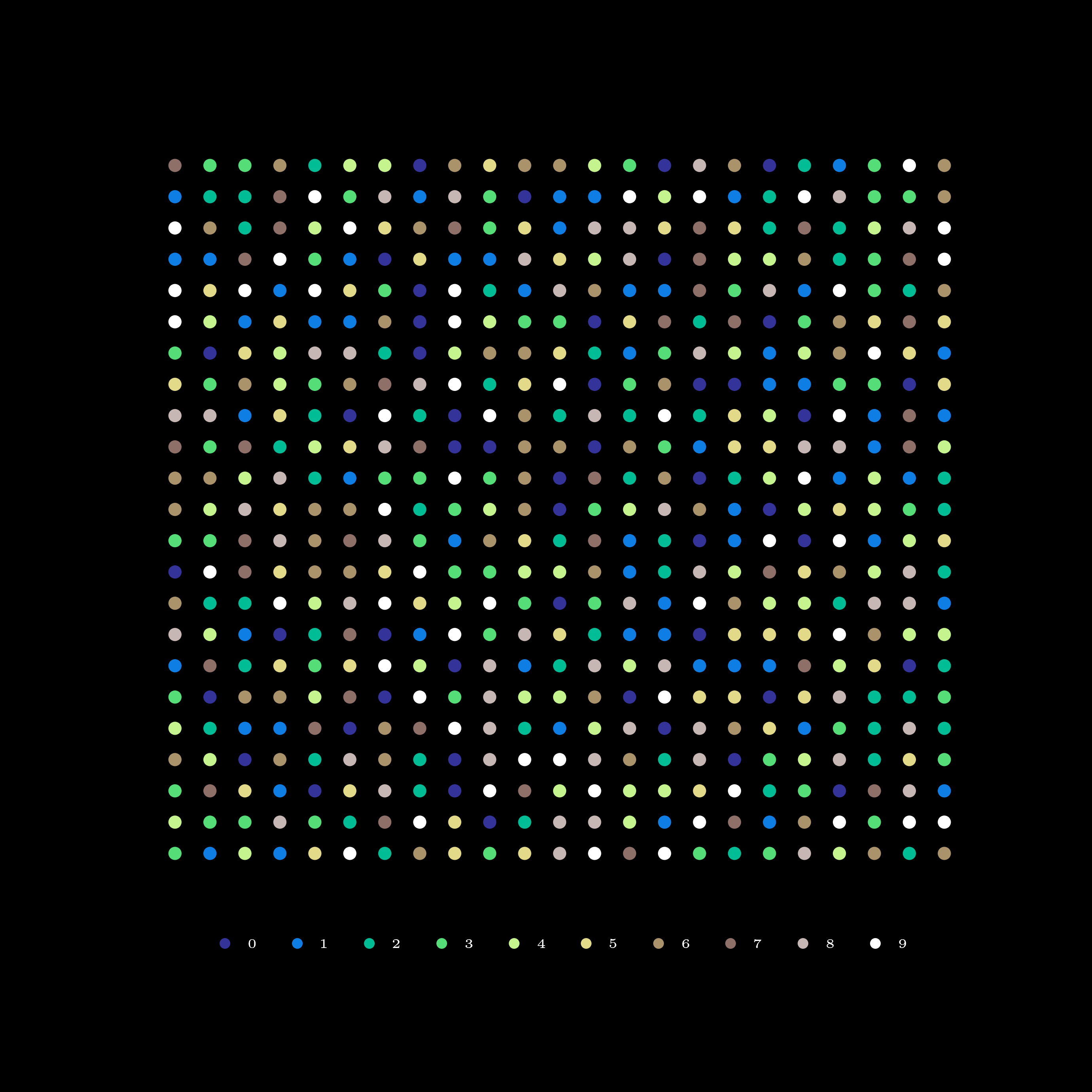
To visualize digits generated from the above snippet, the $n$ digits are laid out on a $r \times c$ evenly-spaced mesh grid and their values are used to fill the colors of the points on the grid. The colors are taken from a discrete color map of size 10:

def discrete_cmap(N, base_cmap=None):
    """Create an N-bin discrete colormap from the specified input map from:
    https://gist.github.com/jakevdp/91077b0cae40f8f8244a
    By Jake VanderPlas
    License: BSD-style
    """
 
    # Note that if base_cmap is a string or None, you can simply do
    #    return plt.cm.get_cmap(base_cmap, N)
    # The following works for string, None, or a colormap instance:
 
    base = plt.cm.get_cmap(base_cmap)
    color_list = base(np.linspace(0, 1, N))
    cmap_name = base.name + str(N)
    return color_list, base.from_list(cmap_name, color_list, N)
 
if __name__ == '__main__':
    ...
    ...
    r, c = np.shape(pi_digits) # pi digits in meshgrid
    x, y = np.meshgrid(np.arange(r), np.arange(c))
 
    # initialize figure
    fig, axes = plt.subplots(figsize=(8, 4))
 
    color_list, dcmap = discrete_cmap(n, "terrain")
 
    # swap y and x
    scat = axes.scatter(
      y, x, c=digits[x, y], s=3, cmap=dcmap
    )
 
    axes.axis('off')
    legend1 = axes.legend(*scat.legend_elements(), loc='upper center',
                          bbox_to_anchor=(0.5, 1.1), ncol=n, fontsize=4.5,
                          markerscale=.5, frameon=False)
    axes.add_artist(legend1)
 
    # show figure
    plt.tight_layout()
    plt.show()

Above code snippet should be able to reproduce something along these lines

_{23x23 meshgrid of the first 529 pi digits. Click to enlarge image.}

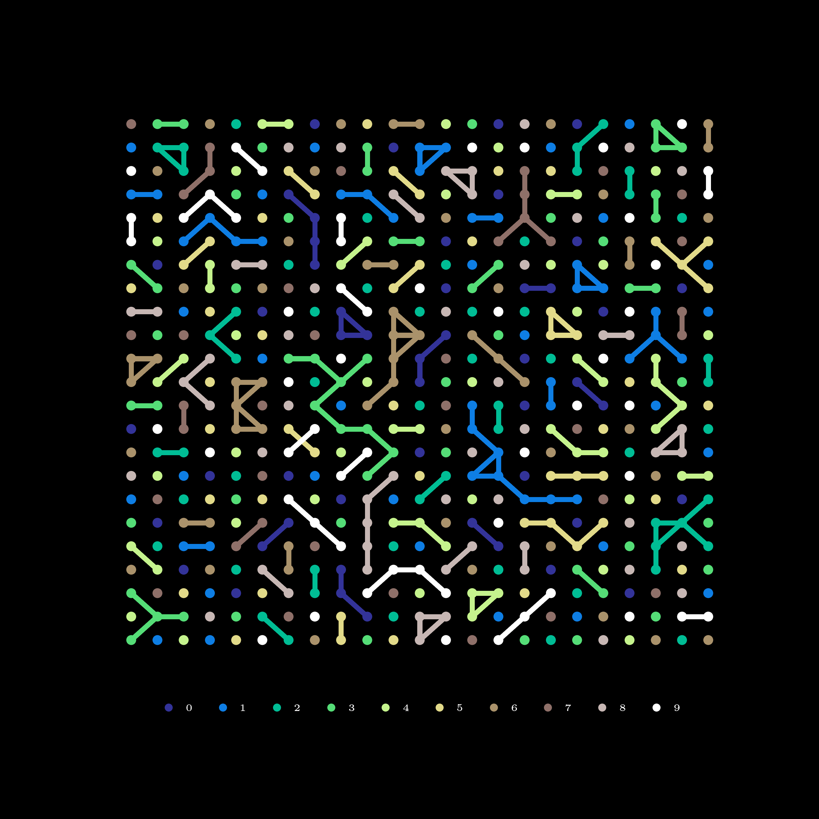
Nearest-neighbor connections

In the original poster, the same-valued digits that are one point away from each other in either direction are connected with edges. For example, for a $3$ by $3$ grid with the following $\pi$ digits

the 1s across the diagonal from the first row and second row will be connected. Similarly, the 6s along the third row.

To achieve this effect , we need to able to find the indices of the connected clusters across the whole grid and use them to draw the edges between the corresponding grid points. Scouring around the internet, I found that such a computation is related to a concept in graph theory, which is the concept of connected components of an undirected graph. Finding the connected components of all the digits from $0-9$ across the grid will give us what we want.

At first sight, this seemed like a daunting task and I was apprehensive of whether a vanilla python implementation would be up to the task. However, it turns out this task is related to labeling components in a pixel array. Consider the following $3 \times 3$ pixel array.

The four 1s in the grid would be deemed as a label/component and we would have only one component in the grid. The scipy library has a high performance C implementation, scipy.ndimage.label, to label the components and subsequently extract their indices. This method also considers isolated groups (1s surrounded by 0s in all directions) as connected components. However, one can filter out isolated groups from the original array as done here. Putting everything together, we can produce the visuals below:

_{23 by 23 meshgrid of the first 529 pi digits with matching nearest-neighbor connections. Click to enlarge image.}

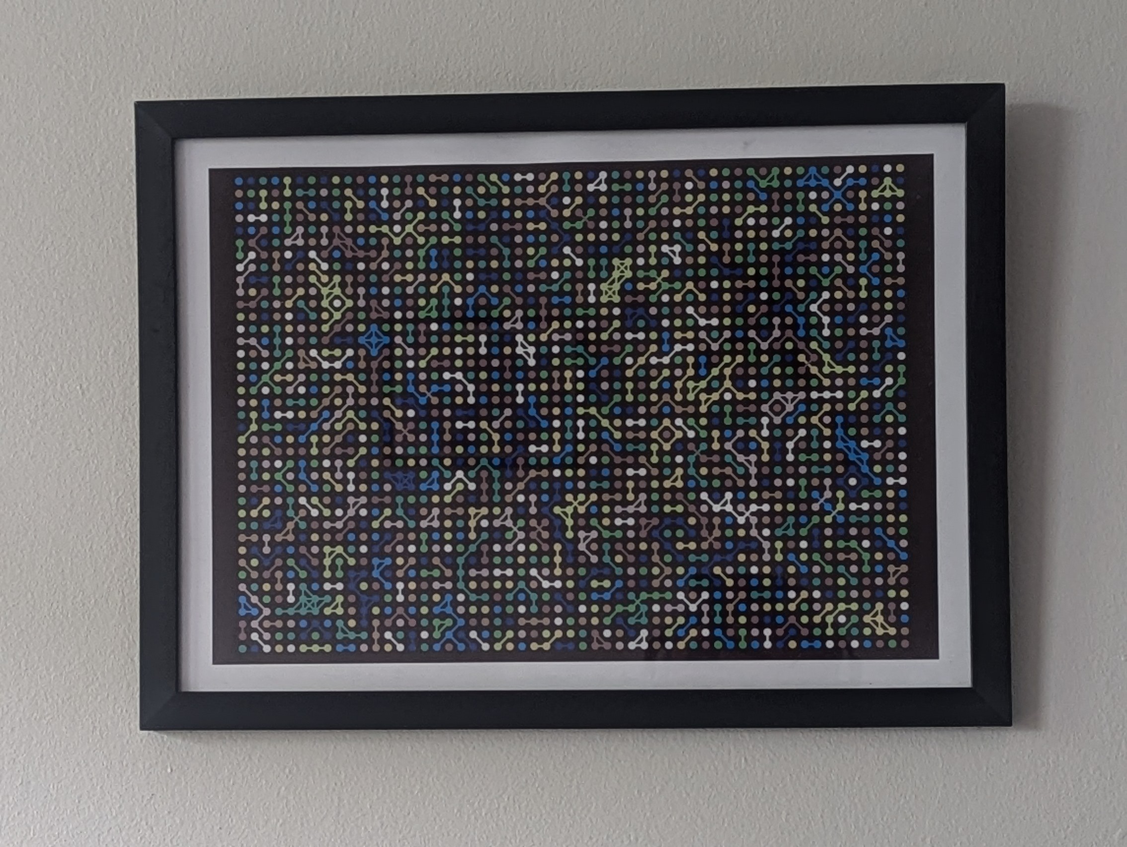
The higher quality images and the complete source code can be found here. Make your own, print and frame in your living room

_{39 by 55 Pi Digits Meshgrid matching nearest-neighbor connections in the living room. Click to enlarge image.}

Fin.